I was recently asked to deliver a session on Earth Science for kids. My daughter goes to an after-school science program at Max Science where they teach science with unique and fun hands-on experiments. They wanted to do an interactive session to introduce the kids to Earth Science and asked if I could deliver a guest talk for their kids in Grades 1 to 4. I loved the idea and developed a module titled The Science of Satellites to introduce the magic of remote sensing to primary school kids. The session ended up being a lot of fun, for the kids and me. In this post, I want to go through the materials and my experience teaching this session.
All the content developed for this session – including high-resolution graphics – is available freely for download. Scroll to the bottom to find the download link.
The 1.5 hour session was split into 3 parts:
Part 1 Guess the Place A game to guess the place from satellite images
Part 2: The Science of Satellites Learning what satellites do and how can you build and launch a satellite
Part 3: Your Name from Space An activity where kids create their from letters seen from satellite images.
In this post, we will learn how to build a regression model in Google Earth Engine and use it to estimate total above ground biomass using openly available Earth Observation datasets.
NASA’s Global Ecosystem Dynamics Investigation (GEDI) mission collects LIDAR measurements along ground transects at 30m spatial resolution at 60m intervals. The GEDI waveform captures the vertical distribution of vegetation structure and is used to derive estimates of Aboveground Biomass Density (AGBD) at each sample. These sample estimates of AGBD are useful but since they are point measurements – you cannot directly use them to calculate total aboveground biomass for a region. We can use other satellite datasets to build a regression model using the GEDI samples to map and quantify the biomass in a region.
Regression Workflow
This article shows how we can build and run the entire workflow in Earth Engine – from pre-processing to building a regression model to running the predictions. You will also learn some advanced techniques and best practices such as:
How to fuse datasets of different resolutions by using setDefaultProjection() and reduceResolution() to align them to a common grid.
How to sample pixels from rasters with sparse data efficiently and precisely by leveraging the image mask using stratifiedSample().
How to split your workflow into separate steps and use Exports to avoid user memory limit exceeded or computation timed-out errors.
ISRO recently released the full archive of medium and low-resolution Earth Observation dataset to the public. This includes the imagery from LISS-IV camera aboard ResourceSat-2 and ResourceSat-2A satellites. This is currently the highest spatial resolution imagery available in the public domain for India. In this post, I want to cover the steps required to download the imagery and apply the pre-processing steps required to make this data ready for analysis – specifically how to programmatically convert the DN values to TOA Reflectance. We will use modern Python libraries such as XArray, rioxarray, and dask – which allow use to seamlessly work with large datasets and use all the available compute power on your machine.
Dynamic World is a new landcover product developed by Google and World Resources Institute (WRI). It is a unique dataset that is designed to make it easy for users to develop locally relevant landcover classification easily. Contrary to other landcover products which try to classify the pixels into a single class – the Dynamic World (DW) model gives you the probability of the pixel belonging to each of the 9 different landcover classes. The full dataset contains the DW class probabilities for every Sentinel-2 scene since 2015 having <35% cloud-cover. It is also updated continuously with detections from new Sentinel-2 scenes as soon as they are available. This makes DW ideal for change detection and monitoring applications.
A key fact about this dataset is that Dynamic World is not a ready-to-use landcover product. Users are expected to fine-tune the output of DW with local knowledge into a final landcover product. Since DW provides per-pixel probabilities generated by a Fully Convolutional Neural Network (FCNN) model, a lot of difficult problems encountered in classifying remotely sensed imagery are addressed already and allows users to refine it with a relatively simple model (such as Random Forest) with small amount of local training data.
A good mental model to use for Dynamic World is to not think of it as landcover product but as a dataset that provides 9 additional bands of landcover related information for each Sentinel-2 image that can be refined to build a locally relevant classification or change detection model.
As seen in the mangrove classification example, using the Dynamic World probability bands as input to a supervised classification model can help you generate a more accurate landcover map in less amount of time. It also eliminates the need for post-processing the results.
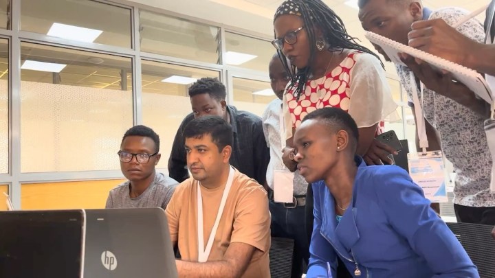
To test this concept and explore the potential of this new dataset in developing locally relevant landcover maps – I partnered with Google and WRI to develop a training workshop and host a 5-day “Mapathon” with participants of diverse backgrounds. The event was a mix of hands-on workshop along with hackathon-style group projects to use Dynamic World for a real-world application.
The workshop was hosted by Regional Centre for Mapping of Resources for Development (RCMRD) in Nairobi, Kenya. You can read more about the event in this article. I and Elise Mazur from WRI also gave a talk about our experience at Geo for Good 2023.
In this post, I want to share more technical details about the workshop materials and code for projects for those who may want to use Dynamic World for their own applications.
Extracting building footprints from high-resolution imagery is a challenging task. Fortunately we now have access to ready-to-use building footprints dataset extracted using state-of-the-art ML techniques. Google’s Open Buildings project has mapped and extracted 1.8 billion buildings in Africa, South Asia, South-East Asia, Latin America and the Caribbean. Microsoft’s Global ML Building Footprints project has made over 1.24 billion building footprints available from most regions of the world.
Update: VIDA has released the most comprehensive buildings dataset by combining both Google and Microsoft building footprint dataset. This dataset is available in Google Earth Engine via the GEE Community Catalog.
Given the availability of these datasets, we can now analyze them to create derivative products. In this post, we will learn how to access these datasets and compute the aggregate count of buildings within a regular grid using Google Earth Engine. We will then export the grid as a shapefile and create a building density map in QGIS.
An important concept in spatial statistics is pixel weights. When calculating pixel statistics with a polygon, partial pixel overlaps are treated differently by different packages and you need to understand this to evaluate the accuracy of your results. Consider the following image. What is the correct answer?
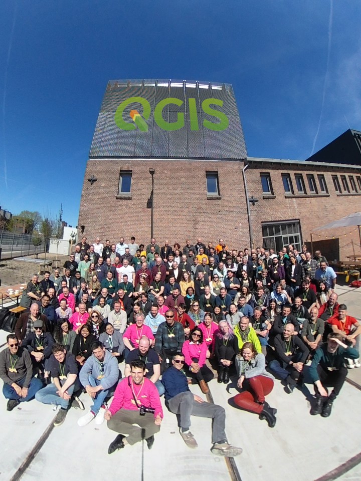
A long awaited community event that happened after a break of 3 years. The conference was attended by over 200 people from across the world. I got a chance to participate and meet many of QGIS community members in-person.
Conference Group Photo
In this post, I hope to share some of my insights and resources from the conference.
In this article, I will outline a method for extracting shoreline from satellite images in Google Earth Engine. This method is scalable and automatically extracts the coastline as a vector polyline. The full code link is available at the end of the post.
UPDATE: The post now includes tidal-phase filtering using HYCOM Data.
The method involves the following steps
Create a Cloud-free Composite Image from images collected during the same tidal phase
Extract All Waterbodies
Remove Inland Water and Small Islands
Convert Raster to Vector
Simplify and Extract Coastline
Video Demonstration of the Script
We will go through the details of each step and review the Google Earth Engine API code required to achieve the results.
Modern versions of QGIS comes with a handy command-line utility called qgis_process. This allows you to access and run any Processing Tool, Script or Model from the Processing Toolbox on a terminal. This is very useful for automation since it doesn’t require you to open QGIS or manually click buttons. You can run the algorithms in a headless-mode and even schedule them to run them at specific times.
This post covers the following topics
How to launch qgis_process command on Windows, Mac and Linux.
How to find the parameters and values for each algorithm and build your command
Example showing how to do a spatial join on the command-line using the Join Attributes by Location algorithm
Example showing how to run a model on the command line to automate a complex workflow
Want to follow along? You can download the data package containing all the datasets used in this post. Before running each command, make sure to replace the paths in the commands with the paths on your computer.
If you are like me, you have a lot of assets uploaded to Earth Engine. As you upload more and more assets, managing this data becomes quite a cumbersome task. Earth Engine provides a handy Command-Line Tool that helps with asset management. While the command-line tool is very useful, it falls short when it comes to bulk data management tasks.
What if you want to rename an ImageCollection? You will need to manually move each child image to a new collection. If you wanted to delete assets matching certain keywords, you’ll need to write a custom shell script. If you are running low on your asset quota and want to delete large assets, there is no direct way to list large assets. Fortunately, the Earth Engine Python Client API comes with a handy ee.data module that we can leverage to write custom scripts. In this post, I will cover the following use cases with full python scripts that can be used by anyone to manage their assets:
How to get a list of all your assets (including folders/sub-folders/collections)
How to share all assets in a folder
How to find the quota consumed by each asset and find large assets
How to rename ImageCollections
How to delete ImageCollections
The post explains each use-case with code snippets. If you want to just grab the scripts, they are linked at the end of the post.