Spatial indexing methods help speed up spatial queries. Most GIS software and databases provide a mechanism to compute and use spatial index for your data layers. QGIS as well as PostGIS use a spatial indexing scheme based on R-Tree data structure – which creates a hierarchical tree using bounding boxes of geometries. This is quite efficient and results in big speedup in certain types of spatial queries. Check out Spatial Indexing section of my course Advanced QGIS where I show how to use R-Tree based Spatial index in QGIS.

If you use Python for geoprocesisng, the GeoPandas library also provides an easy to use implementation of R-Tree based spatial index using the .sidex attribute. University of Helsinki’s AutoGIS course has an excellent example of using spatial index with geopandas.

In this post, I want to talk about another spatial indexing system called H3.

This open-source indexing system was created by Uber and uses hexagonal grid cells. This system is akin to another cell based indexing system called S2 – which was developed at Google. Both of these system provide a way to turn a coordinate on earth into a cell id that maps to a hexagonal or rectangular grid cell at a specific resolution. These cell ids have unique properties such as nearby cells have similar ids and you can find parent cells by truncating their length. These properties make operations such as aggregating data, finding nearby objects, measuring distances very fast.

In this post, I will show you how to create a point density map using geopandas and h3-py libraries in Python.

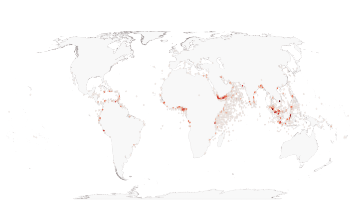
National Geospatial-Intelligence Agency’s Maritime Safety Information portal provides a shapefile of all incidents of maritime piracy in the form on Anti-shipping Activity Messages.

The data comes as a zip file ASAM_shp.zip. The actual data layer is a shapefile is ASAM_events.shp which is inside a folder ASAM_data_download. The dataset contains 8000+ point locations across the globe where piracy incidents have been recorded. Here’s what the raw point layer looks as visualized in QGIS.

We will create a density map by aggregating the incident points over a hexagonal grid provided by H3. We start by importing the libraries.

import geopandas as gpd
from h3 import h3

GeoPandas allow is to read the data layer from a zip file directly.

zipfile = 'zip://ASAM_shp.zip!ASAM_data_download/ASAM_events.shp'
incidents = gpd.read_file(zipfile)

H3 library has 15 levels of resolution. This table shows details of each level. We choose Level 3 which results in a grid size of approximately 100km. The function lat_lng_to_h3 converts a location’s coordinates into an H3 id of the chosen level. We add a column called h3 with the H3 grid id for the point at level 3.

h3_level = 3

def lat_lng_to_h3(row):
    return h3.geo_to_h3(
      row.geometry.y, row.geometry.x, h3_level)

incidents['h3'] = incidents.apply(lat_lng_to_h3, axis=1)

Now the fun part. Since all points that fall in a grid cell will have the same id, we can simply aggregate all rows with the same grid id to find all points that fall in the grid polygon. So by using the grid based indexing system – a complex spatial ‘point-in-polygon‘ operation becomes a simple aggregation over a table. We use Panda’s groupby function on the h3 column and add a new column count to the output with the number of rows for each H3 id.

counts = incidents.groupby(['h3']).h3.agg('count').to_frame('count').reset_index()

We now know the number of piracy incidents for each grid cell. To visualize the results or export it to a GIS, we need to convert the H3 cell ids to a geometry. The h3_to_geo_boundary function takes a H3 key and returns a list of coordinates that form the hexagonal cell. Since GeoPandas uses shapely library for constructing geometries, we convert the list of coordinates to a shapely Polygon object. Note the optional second argument to the h3_to_geo_boundary function which we have set to True which returns the coordinates in the (x,y) order compared to default (lat,lon)

from shapely.geometry import Polygon

def add_geometry(row):
    points = h3.h3_to_geo_boundary(
      row['h3'], True)
    return Polygon(points)

counts['geometry'] = counts.apply(add_geometry, axis=1)

We turn the dataframe to a GeoDataframe with the CRS EPSG:4326 (WGS84 Latitude/Longitude) and write it to a geopackage.

gdf = gpd.GeoDataFrame(counts, crs='EPSG:4326')
output_filename = 'gridcounts.gpkg'
gdf.to_file(driver='GPKG', filename=output_filename)

The gridcounts.gpkg can be opened and visualized in QGIS. Here’s the layer showing the resulting hexbin map showing the piracy hotspots around the world.

The whole process from reading the input to creating the aggregated grid layer takes just over 2 seconds. Compare that to a QGIS model using spatial index which takes at least 5x of that. H3 is uniquely suited for such spatial aggregations and is very fast.

The code and dataset used in this post is available on my Github Repository. You can also run the Jupyter Notebook live in Binder.

Want to learn Python for Spatial Analysis? Check out my course Python Foundation for Spatial Analysis.